As I outlined in my previous blog post on How to clean up network traffic logs, I have been working with the VAST 2013 traffic logs. Today I am going to show you can load the traffic logs into Impala (with a parquet table) for very quick querying.
First off, Impala is a real-time search engine for Hadoop (i.e., Hive/HDFS). So, scalable, distributed, etc. In the following I am assuming that you have Impala installed already. If not, I recommend you use the Cloudera Manager to do so. It’s pretty straight forward.
First we have to load the data into Impala, which is a two step process. We are using external tables, meaning that the data will live in files on HDFS. What we have to do is getting the data into HDFS first and then loading it into Impala:
$ sudo su - hdfs
$ hdfs dfs -put /tmp/nf-chunk*.csv /user/hdfs/data
We first become the hdfs user, then copy all of the netflow files from the MiniChallenge into HDFS at /user/hdfs/data. Next up we connect to impala and create the database schema:
$ impala-shell
create external table if not exists logs (
	TimeSeconds double,
	parsedDate timestamp,
	dateTimeStr string,
	ipLayerProtocol int,
	ipLayerProtocolCode string,
	firstSeenSrcIp string,
	firstSeenDestIp string,
	firstSeenSrcPort int,
	firstSeenDestPor int,
	moreFragment int,
	contFragment int,
	durationSecond int,
	firstSeenSrcPayloadByte bigint,
	firstSeenDestPayloadByte bigint,
	firstSeenSrcTotalByte bigint,
	firstSeenDestTotalByte bigint,
	firstSeenSrcPacketCoun int,
	firstSeenDestPacketCoun int,
	recordForceOut int)
row format delimited fields terminated by ',' lines terminated by '\n'
location '/user/hdfs/data/';
Now we have a table called ‘logs’ that contains all of our data. We told Impala that the data is comma separated and told it where the data files are. That’s already it. What I did on my installation is leveraging the columnar data format of Impala to speed queries up. A lot of analytic queries don’t really suit the row-oriented manner of databases. Columnar orientation is much more suited. Therefore we are creating a Parquet-based table:
create table pq_logs like logs stored as parquetfile;
insert overwrite table pq_logs select * from logs;
The second command is going to take a bit as it loads all the data into the new Parquet table. You can now issues queries against the pq_logs table and you will get the benefits of a columnar data store:
select distinct firstseendestpor from pq_logs where morefragment=1;
Have a look at my previous blog entry for some more queries against this data.
I have spent some significant time with the VAST 2013 Challenge. I have been part of the program committee for a couple of years now and have seen many challenge submissions. Both good and bad. What I noticed with most submissions is that they a) didn’t really understand network data, and b) they didn’t clean the data correctly. If you wanna follow along my analysis, the data is here: Week 1 – Network Flows (~500MB)
Also check the follow-on blog post on how to load data into a columnar data store in order to work with it.
Let me help with one quick comment. There is a lot of traffic in the data that seems to be involving port 0:
$ cat nf-chunk1-rev.csv | awk -F, '{if ($8==0) print $0}'
1364803648.013658,2013-04-01 08:07:28,20130401080728.013658,1,OTHER,172.10.0.6,
172.10.2.6,0,0,0,0,1,0,0,222,0,3,0,0
Just because it says port 0 in there doesn’t mean it’s port 0! Check out field 5, which says OTHER. That’s the transport protocol. It’s not TCP or UDP, so the port is meaningless. Most likely this is ICMP traffic!
On to another problem with the data. Some of the sources and destinations are turned around in the traffic. This happens with network flow collectors. Look at these two records:
1364803504.948029,2013-04-01 08:05:04,20130401080504.948029,6,TCP,172.30.1.11,
10.0.0.12,9130,80,0,0,0,176,409,454,633,5,4,0
1364807428.917824,2013-04-01 09:10:28,20130401091028.917824,6,TCP,172.10.0.4,
172.10.2.64,80,14545,0,0,0,7425,0,7865,0,8,0,0
The first one is totally legitimate. The source port is 9130, the destination 80. The second record, however, has the source and destination turned around. Port 14545 is not a valid destination port and the collector just turned the information around.
The challenge is on you now to find which records are inverted and then you have to flip them back around. Here is what I did in order to find the ones that were turned around (Note, I am only using the first week of data for MiniChallenge1!):
select firstseendestport, count(*) c from logs group by firstseendestport order
 by c desc limit 20;
| 80               | 41229910 |
| 25               | 272563   |
| 0                | 119491   |
| 123              | 95669    |
| 1900             | 68970    |
| 3389             | 58153    |
| 138              | 6753     |
| 389              | 3672     |
| 137              | 2352     |
| 53               | 955      |
| 21               | 767      |
| 5355             | 311      |
| 49154            | 211      |
| 464              | 100      |
| 5722             | 98       |
...
What I am looking for here are the top destination ports. My theory being that most valid ports will show up quite a lot. This gave me a first candidate list of ports. I am looking for two things here. First, the frequency of the ports and second whether I recognize the ports as being valid. Based on the frequency I would put the ports down to port 3389 on my candidate list. But because all the following ones are well known ports, I will include them down to port 21. So the first list is:
80,25,0,123,1900,3389,138,389,137,53,21
I’ll drop 0 from this due to the comment earlier!
Next up, let’s see what the top source ports are that are showing up.
| firstseensrcport | c       |
+------------------+---------+
| 80               | 1175195 |
| 62559            | 579953  |
| 62560            | 453727  |
| 51358            | 366650  |
| 51357            | 342682  |
| 45032            | 288301  |
| 62561            | 256368  |
| 45031            | 227789  |
| 51359            | 180029  |
| 45033            | 157071  |
| 0                | 119491  |
| 45034            | 117760  |
| 123              | 95622   |
| 1984             | 81528   |
| 25               | 19646   |
| 138              | 6711    |
| 137              | 2288    |
| 2024             | 929     |
| 2100             | 927     |
| 1753             | 926     |
See that? Port 80 is the top source port showing up. Definitely a sign of a source/destination confusion. There are a bunch of others from our previous candidate list showing up here as well. All records where we have to turn source and destination around. But likely we are still missing some ports here.
Well, let’s see what other source ports remain:
select firstseensrcport, count(*) c from pq_logs2 group by firstseensrcport
having firstseensrcport<1024 and firstseensrcport not in (0,123,138,137,80,25,53,21)
order by c desc limit 10
+------------------+--------+
| firstseensrcport | c      |
+------------------+--------+
| 62559            | 579953 |
| 62560            | 453727 |
| 51358            | 366650 |
| 51357            | 342682 |
| 45032            | 288301 |
| 62561            | 256368 |
| 45031            | 227789 |
| 51359            | 180029 |
| 45033            | 157071 |
| 45034            | 117760 |
Looks pretty normal. Well. Sort of, but let’s not digress. But lets try to see if there are any ports below 1024 showing up. Indeed, there is port 20 that shows, totally legitimate destination port. Let’s check out the. Pulling out the destination ports for those show nice actual source ports:
+------------------+------------------+---+
| firstseensrcport | firstseendestport| c |
+------------------+------------------+---+
| 20               | 3100             | 1 |
| 20               | 8408             | 1 |
| 20               | 3098             | 1 |
| 20               | 10129            | 1 |
| 20               | 20677            | 1 |
| 20               | 27362            | 1 |
| 20               | 3548             | 1 |
| 20               | 21396            | 1 |
| 20               | 10118            | 1 |
| 20               | 8407             | 1 |
+------------------+------------------+---+
Adding port 20 to our candidate list. Now what? Let’s see what happens if we look at the top ‘connections’:
select firstseensrcport,
firstseendestport, count(*) c from pq_logs2 group by firstseensrcport,
firstseendestport having firstseensrcport not in (0,123,138,137,80,25,53,21,20,1900,3389,389)
and firstseendestport not in (0,123,138,137,80,25,53,21,20,3389,1900,389)
order by c desc limit 10
+------------------+------------------+----+
| firstseensrcport | firstseendestpor | c  |
+------------------+------------------+----+
| 1984             | 4244             | 11 |
| 1984             | 3198             | 11 |
| 1984             | 4232             | 11 |
| 1984             | 4276             | 11 |
| 1984             | 3212             | 11 |
| 1984             | 4247             | 11 |
| 1984             | 3391             | 11 |
| 1984             | 4233             | 11 |
| 1984             | 3357             | 11 |
| 1984             | 4252             | 11 |
+------------------+------------------+----+
Interesting. Looking through the data where the source port is actually 1984, we can see that a lot of the destination ports are showing increasing numbers. For example:
| 1984             | 2228             | 172.10.0.6     | 172.10.1.118    |
| 1984             | 2226             | 172.10.0.6     | 172.10.1.147    |
| 1984             | 2225             | 172.10.0.6     | 172.10.1.141    |
| 1984             | 2224             | 172.10.0.6     | 172.10.1.115    |
| 1984             | 2223             | 172.10.0.6     | 172.10.1.120    |
| 1984             | 2222             | 172.10.0.6     | 172.10.1.121    |
| 1984             | 2221             | 172.10.0.6     | 172.10.1.135    |
| 1984             | 2220             | 172.10.0.6     | 172.10.1.126    |
| 1984             | 2219             | 172.10.0.6     | 172.10.1.192    |
| 1984             | 2217             | 172.10.0.6     | 172.10.1.141    |
| 1984             | 2216             | 172.10.0.6     | 172.10.1.173    |
| 1984             | 2215             | 172.10.0.6     | 172.10.1.116    |
| 1984             | 2214             | 172.10.0.6     | 172.10.1.120    |
| 1984             | 2213             | 172.10.0.6     | 172.10.1.115    |
| 1984             | 2212             | 172.10.0.6     | 172.10.1.126    |
| 1984             | 2211             | 172.10.0.6     | 172.10.1.121    |
| 1984             | 2210             | 172.10.0.6     | 172.10.1.172    |
| 1984             | 2209             | 172.10.0.6     | 172.10.1.119    |
| 1984             | 2208             | 172.10.0.6     | 172.10.1.173    |
That would hint at this guy being actually a destination port. You can also query for all the records that have the destination port set to 1984, which will show that a lot of the source ports in those connections are definitely source ports, another hint that we should add 1984 to our list of actual ports. Continuing our journey, I found something interesting. I was looking for all connections that don’t have a source or destination port in our candidate list and sorted by the number of occurrences:
+------------------+------------------+---+
| firstseensrcport | firstseendestport| c |
+------------------+------------------+---+
| 62559            | 37321            | 9 |
| 62559            | 36242            | 9 |
| 62559            | 19825            | 9 |
| 62559            | 10468            | 9 |
| 62559            | 34395            | 9 |
| 62559            | 62556            | 9 |
| 62559            | 9005             | 9 |
| 62559            | 59399            | 9 |
| 62559            | 7067             | 9 |
| 62559            | 13503            | 9 |
| 62559            | 30151            | 9 |
| 62559            | 23267            | 9 |
| 62559            | 56184            | 9 |
| 62559            | 58318            | 9 |
| 62559            | 4178             | 9 |
| 62559            | 65429            | 9 |
| 62559            | 32270            | 9 |
| 62559            | 18104            | 9 |
| 62559            | 16246            | 9 |
| 62559            | 33454            | 9 |
This is strange in so far as this source port seems to connect to totally random ports, but not making any sense. Is this another legitimate destination port? I am not sure. It’s way too high and I don’t want to put it on our list. Open question. No idea at this point. Anyone?
Moving on without this 62559, we see the same behavior for 62560 and then 51357 and 51358, as well as 45031, 45032, 45033. And it keeps going like that. Let’s see what the machines are involved in this traffic. Sorry, not the nicest SQL, but it works:
.
select firstseensrcip, firstseendestip, count(*) c
from pq_logs2 group by firstseensrcip, firstseendestip,firstseensrcport
having firstseensrcport in (62559, 62561, 62560, 51357, 51358)
order by c desc limit 10
+----------------+-----------------+-------+
| firstseensrcip | firstseendestip | c     |
+----------------+-----------------+-------+
| 10.9.81.5      | 172.10.0.40     | 65534 |
| 10.9.81.5      | 172.10.0.4      | 65292 |
| 10.9.81.5      | 172.10.0.4      | 65272 |
| 10.9.81.5      | 172.10.0.4      | 65180 |
| 10.9.81.5      | 172.10.0.5      | 65140 |
| 10.9.81.5      | 172.10.0.9      | 65133 |
| 10.9.81.5      | 172.20.0.6      | 65127 |
| 10.9.81.5      | 172.10.0.5      | 65124 |
| 10.9.81.5      | 172.10.0.9      | 65117 |
| 10.9.81.5      | 172.20.0.6      | 65099 |
+----------------+-----------------+-------+
Here we have it. Probably an attacker :). This guy is doing not so nice things. We should exclude this IP for our analysis of ports. This guy is just all over.
Now, we continue along similar lines and find what machines are using port 45034, 45034, 45035:
select firstseensrcip, firstseendestip, count(*) c
from pq_logs2 group by firstseensrcip, firstseendestip,firstseensrcport
having firstseensrcport in (45035, 45034, 45033)  order by c desc limit 10
+----------------+-----------------+-------+
| firstseensrcip | firstseendestip | c     |
+----------------+-----------------+-------+
| 10.10.11.15    | 172.20.0.15     | 61337 |
| 10.10.11.15    | 172.20.0.3      | 55772 |
| 10.10.11.15    | 172.20.0.3      | 53820 |
| 10.10.11.15    | 172.20.0.2      | 51382 |
| 10.10.11.15    | 172.20.0.15     | 51224 |
| 10.15.7.85     | 172.20.0.15     | 148   |
| 10.15.7.85     | 172.20.0.15     | 148   |
| 10.15.7.85     | 172.20.0.15     | 148   |
| 10.7.6.3       | 172.30.0.4      | 30    |
| 10.7.6.3       | 172.30.0.4      | 30    |
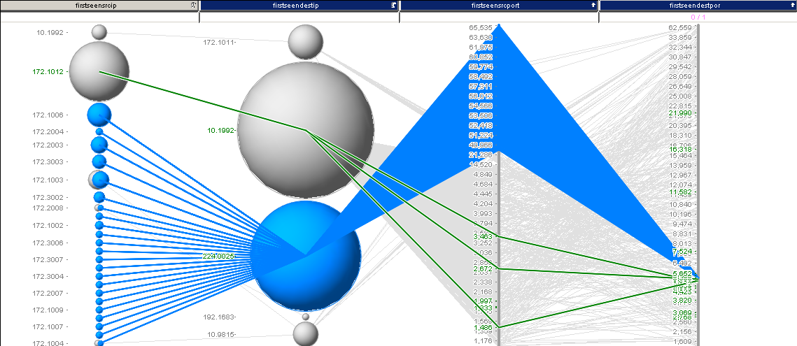
We see one dominant IP here. Probably another ‘attacker’. So we exclude that and see what we are left with. Now, this is getting tedious. Let’s just visualize some of the output to see what’s going on. Much quicker! And we only have 36970 records unaccounted for.

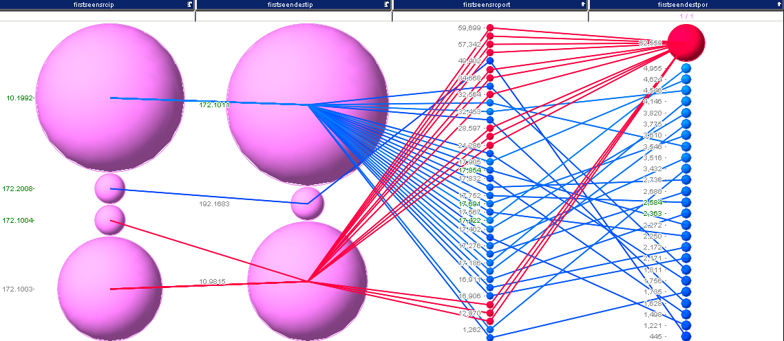
What you can see is the remainder of traffic. Very quickly we see that there is one dominant IP address. We are going to filter that one out. Then we are left with this:
I selected some interesting traffic here. Turns out, we just found another destination port: 5535 for our list. I continued this analysis and ended up with something like 38 records, which are shown in the last image:
I’ll leave it at this for now. I think that’s a pretty good set of ports:
20,21,25,53,80,123,137,138,389,1900,1984,3389,5355
Oh well, if you want to fix your traffic now and turn around the wrong source/destination pairs, here is a hack in perl:
$ cat nf*.csv | perl -F\,\ -ane 'BEGIN {@ports=(20,21,25,53,80,123,137,138,389,1900,1984,3389,5355);
%hash = map { $_ => 1 } @ports; $c=0} if ($hash{$F[7]} && $F[8}>1024)
{$c++; printf"%s,%s,%s,%s,%s,%s,%s,%s,%s,%s,%s,%s,%s,%s,%s,%s,%s,%s,%s",
$F[0],$F[1],$F[2],$F[3],$F[4],$F[6],$F[5],$F[8],$F[7],$F[9],$F[10],$F[11],$F[13],$F[12],
$F[15],$F[14],$F[17],$F[16],$F[18]} else {print $_} END {print "count of revers $c\n";}'
We could have switched to visual analysis way earlier, which I did in my initial analysis, but for the blog I ended up going way further in SQL than I probably should have. The next blog post covers how to load all of the VAST data into a Hadoop / Impala setup.
