August 7, 2018
Join me for my talk about AI and ML in cyber security at BlackHat on Thursday the 9th of August in Las Vegas. I’ll be exploring the topics of artificial intelligence (AI) and machine learning (ML) to show some of the ‘dangerous’ mistakes that the industry (vendors and practitioners alike) are making in applying these concepts in security.
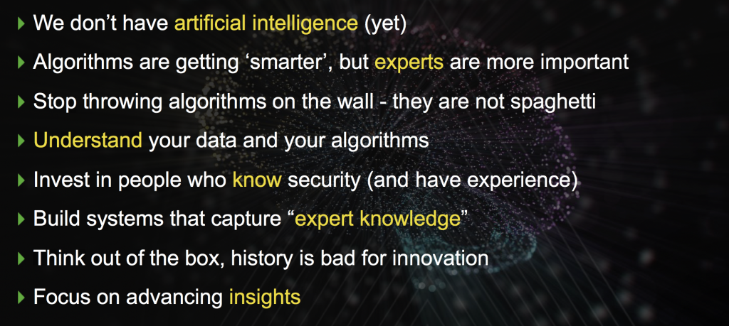
We don’t have artificial intelligence (yet). Machine learning is not the answer to your security problems. And downloading the ‘random’ analytic library to identify security anomalies is going to do you more harm than it helps.
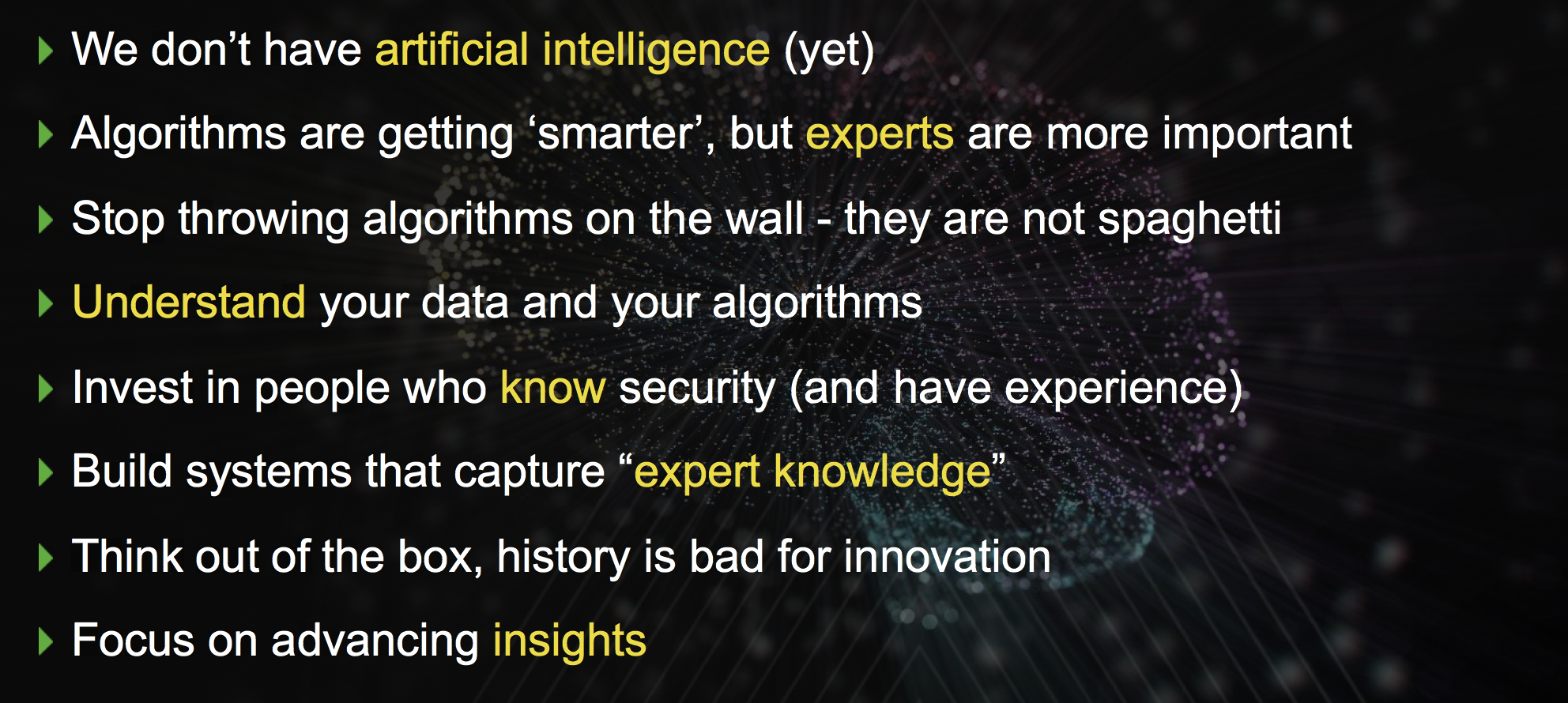
We will explore these accusations and walk away with the following learnings from the talk:
I am exploring these items throughout three sections in my talk: 1) A very quick set of definitions for machine learning, artificial intelligence, and data mining with a few examples of where ML has worked really well in cyber security. Check cybersecuritycourses.com here for an overview of the best cyber security courses available. 2) A closer and more technical view on why algorithms are dangerous. Why it is not a solution to download a library from the Internet to find security anomalies in your data. 3) An example scenario where we talk through supervised and unsupervised machine learning for network traffic analysis to show the difficulties with those approaches and finally explore a concept called belief networks that bear a lot of promise to enhance our detection capabilities in security by leveraging export knowledge more closely. And if you plan to test the the vulnerability of your network, make use of Wifi Pineapple testing tool.

I keep mentioning that algorithms are dangerous. Dangerous in the sense that they might give you a false sense of security or in the worst case even decrease your security quite significantly. Here are some questions you can use to self-assess whether you are ready and ‘qualified’ to use data science or ‘advanced’ algorithms like machine learning or clustering to find anomalies in your data:
- Do you know what the difference is between supervised and unsupervised machine learning?
- Can you describe what a distance function is?
- In data science we often look at two types of data: categorical and numerical. What are port numbers? What are user names? And what are IP sequence numbers?
- In your data set you see traffic from port 0. Can you explain that?
- You see traffic from port 80. What’s a likely explanation of that? Bonus points if you can come up with two answers.
- How do you go about selecting a clustering algorithm?
- What’s the explainability problem in deep learning?
- How do you acquire labeled network data sets (netflows or pcaps)?
- Name three data cleanliness problems that you need to account for before running any algorithms?
- When running k-means, do you have to normalize your numerical inputs?
- Does k-means support categorical features?
- What is the difference between a feature, data field, and a log record?
If you can’t answer the above questions, you might want to rethink your data science aspirations and come to my talk on Thursday to hopefully walk away with answers to the above questions.
Update 8/13/18: Added presentation slides
July 12, 2018
Late June, my alma mater organized an event in Brooklyn with the title: “ETH Meets New York”. The topic of the evening was “Security Technologies Enabling the Future: From Blockchain to IoT”. I was one of the speakers talking about “AI in Practice – What We Learned in Cyber Security”. The video of the talk is available online. It’s a short 10 minutes where I discuss some of the problems with AI in cyber, and outline how expert knowledge is more important than algorithms when it comes to detecting malicious actors in our systems.
Spark your interest? Don’t miss my talk at BlackHat next month where we will have an hour to explore the topics of analytics, machine learning, and artificial intelligence in cyber. I recorded a brief teaser video to help you understand what I will be covering.
ETH meets NY 2018_vimeo1 from ETH Zurich on Vimeo.
A quick summary of the talks can be found in this summary blog post.
March 29, 2018
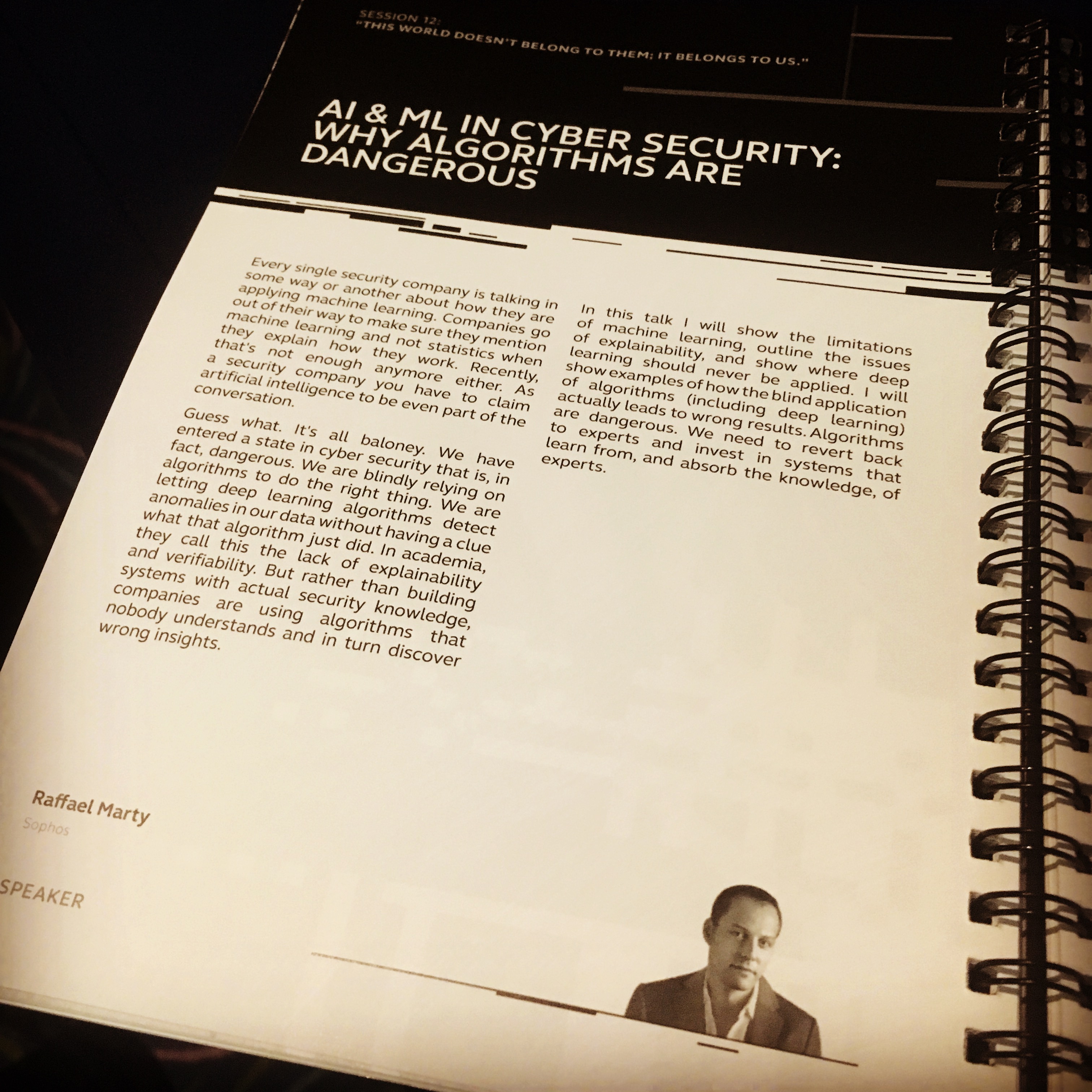
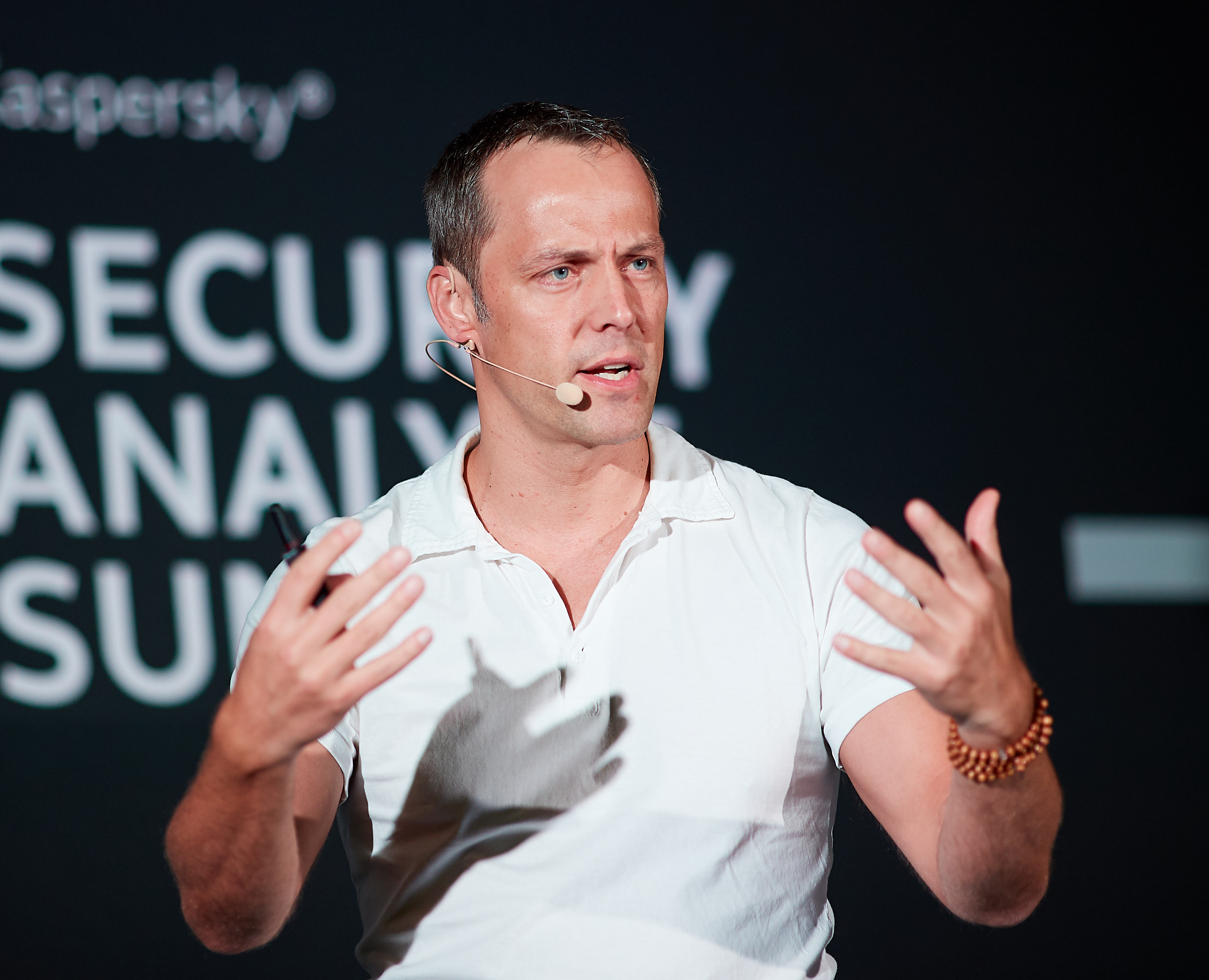
 Another year, another Security Analytics Summit. This year Kaspersky gathered an amazing set of speakers in Cancun, Mexico. I presented on AI & ML in Cyber Security – Why Algorithms Are Dangerous. I was really pleased how well the talk was received and it was super fun to see the storm that emerged on Twitter where people started discussing AI and ML.
Here are a couple of tweets that attendees of my talk tweeted out (thanks everyone!):

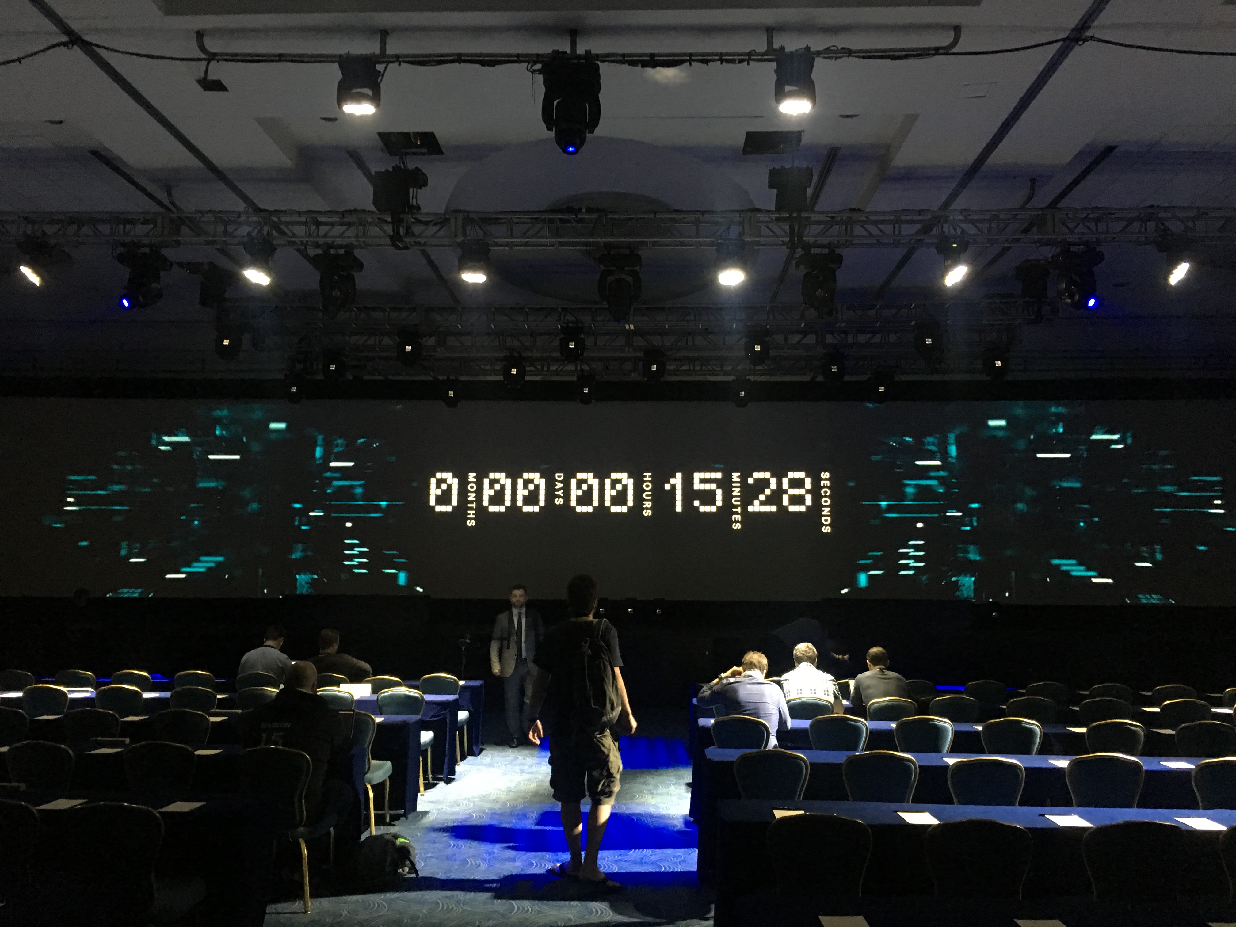
The following are some more impressions from the conference:


And here are the slides:
January 17, 2018
I just read an article on virtual reality (VR) in cyber security and how VR can be used in a SOC.

Image taken from original post
The post basically says that VR helps the SOC be less of an expensive room you have to operate by letting a company take the SOC virtual. Okay. I am buying that argument to some degree. It’s still different to be in the same room with your team, but okay.
Secondly, the article says that it helps tier-1 analysts look at context (I am paraphrasing). So in essence, they are saying that VR helps expand the number of pixels available. Just give me another screen and I am fine. Just having VR doesn’t mean we have the data to drive all of this. If we had it, it would be tremendously useful to show that contextual information in the existing interfaces. We don’t need VR for that. So overall, a non-argument.
There is an entire paragraph of non-sense in the post. VR (over traditional visualization) won’t help monitoring more sources. It won’t help with the analysis of endpoints. etc. Oh boy and “.. greater context and consumable intelligence for the C-suite.” For real? That’s just baloney!
Before we embark on VR, we need to get better at visualizing security data and probably some more advanced cyber security training for employees. Then, at some point, we can see if we want to map that data into three dimensions and whether that will actually help us being more efficient. VR isn’t the silver bullet, just like artificial intelligence (AI) isn’t either.
This is a gem within the article; a contradiction in itself: “More dashboards and more displays are not the answer. But a VR solution can help effectively identify potential threats and vulnerabilities as they emerge for oversight by the blue (defensive) team.” – What is VR other than visualization? If you can show it in three dimensions within some google, can’t you show it in two dimensions on a flat screen?
January 14, 2018
I have been talking about artificial intelligence (AI) and machine learning (ML) in cyber security quite a bit lately. My latest two essays you can find as guest posts on TowardsDataScience and DarkReading.
Following is a summary of the latest AI and ML posts with quick summaries:
I’d love to hear your comments – be that on twitter or as comments on the posts!
December 15, 2017
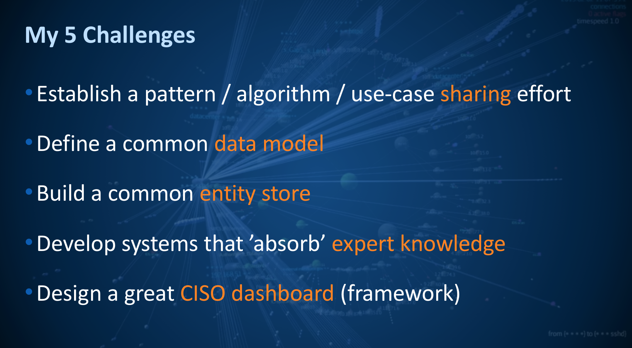
Previously, I started blogging about individual topics and slides from my keynote at ACSAC 2017. The first topic I elaborated on a little bit was An Incomplete Security Big Data History. In this post I want to focus on the last slide in the presentation, where I posed 5 Challenges for security with big data:
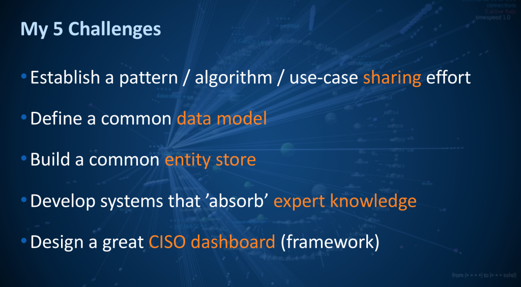
Let me explain and go into details on these challenges a bit more:
- Establish a pattern / algorithm / use-case sharing effort: Part of the STIX standard for exchanging threat intelligence is the capability to exchange patterns. However, we have been notoriously bad at actually doing that. We are exchanging simple indicators of compromise (IOCs), such as IP addresses or domain names. But talk to any company that is using those, and they’ll tell you that those indicators are mostly useless. We have to up-level our detections and engage in patterns; also called TTPs at times: tactics, techniques, and procedures. Those characterize attacker behavior, rather than calling out individual technical details of the attack. Back in the good old days of SIM, we built correlation rules (we actually still do). Problem is that we don’t share them. The default content delivered by the SIMs is horrible (I can say that. I built all of those for ArcSight back in the day). We don’t have a place where we can share our learnings. Every SIEM vendor is trying to do that on their own, but we need to start defining those patterns independent of products. Let’s get going! Who makes the first step?
- Define a common data model: For over a decade, we have been trying to standardize log formats. And we are still struggling. I initially wrote the Common Event Format (CEF) at ArcSight. Then I went to Mitre and tried to get the common event expression (CEE) work off the ground to define a vendor neutral standard. Unfortunately, getting agreement between Microsoft, RedHat, Cisco, and all the log management vendors wasn’t easy and we lost the air force funding for the project. In the meantime I went to work for Splunk and started the common information model (CIM). Then came Apache Spot, which has defined yet another standard (yes, I had my fingers in that one too). So the reality is, we have 4 pseudo standards, and none is really what I want. I just redid some major parts over here at Sophos (I hope I can release that at some point).
Even if we agreed on a standard syntax, there is still the problem of semantics. How do you know something is a login event? At ArcSight (and other SIEM vendors) that’s called the taxonomy or the categorization. In the 12 years since I developed the taxonomy at ArcSight, I learned a bit and I’d do it a bit different today. Well, again, we need standards that products implement. Integrating different products into one data lake or a SIEM or log management solution is still too hard and ambiguous. But you can learn doing this if you will look for Fortinet and learn how they do this.
- Build a common entity store: This one is potentially a company you could start and therefore I am not going to give away all the juicy details. But look at cyber security. We need more context for the data we are collecting. Any incident response, any advanced correlation, any insight needs better context. What’s the user that was logged into a system? What’s the role of that system? Who owns it, etc. All those factors are important. Cyber security has an entity problem! How do you collect all that information? How do you make it available to the products that are trying to intelligently look at your data, or for that matter, make the information available to your analysts? First you have to collect the data. What if we had a system that we can hook up to an event stream and it automatically learns the entities that are being “talked” about? Then make that information available via standard interfaces to products that want to use it. There is some money to be made here! Oh, and guess what! By doing this, we can actually build it with privacy in mind. Anonymization built in! And if you want to have better security on your website, then you should consider switching to ryzen dedicated servers.
- Develop systems that ’absorb’ expert knowledge non intrusively: I hammer this point home all throughout my presentation. We need to build systems that absorb expert knowledge. How can we do that without being too intrusive? How do we build systems with expert knowledge? This can be through feedback loops in products, through bayesian belief networks, through simple statistics or rules, … but let’s shift our attention to knowledge and how we make experts by CCTV Melbourne and highly paid security people more efficient.
- Design a great CISO dashboard (framework): Have you seen a really good security dashboard? I’d love to see it (post in the comments?). It doesn’t necessarily have to be for a CISO. Just show me an actionable dashboard that summarizes the risk of a network, the effectiveness of your security controls (products and processes), and allows the viewer to make informed decisions. I know, I am being super vague here. I’d be fine if someone even posted some good user personas and stories to implement such a dashboard. (If you wait long enough, I’ll do it). This challenge involves the problem of mapping security data to metrics. Something we have been discussing for eons. It’s hard. What’s a 10 versus a 5 when it comes to your security posture? Any (shared) progress on this front would help.
What are your thoughts? What challenges would you put out? Am I missing the mark? Or would you share my challenges?
December 11, 2017
You are an enterprise software startup. You are in the security space. Your company is still early, trying to sign its first 10, maybe 40 customers. What should you be doing for marketing? What works? What doesn’t? What approaches yield the biggest return for your investment? These are some questions that I have been pondering lately with startups that I am working with. I decided to do some research among my marketing and startup friends to explore what marketing approaches work for them.
The full posts you can find on my other blog at cryptojail.net. There you will find a discussion of:
- Positioning and value proposition
- Identifying your top 200 prospects
- Defining measurable goals
- Building a killer Web site
- Getting reference customers
- Keeping your marketing fun and unique
- Becoming good at PR
- etc.
And don’t forget about proper advertising and marketing strategies. A good SEO campaign from the best SEO company will give your business the attention it deserves.
Here are the individual posts:
- Startup Marketing
- Get Good at PR
- More PR Activities
December 6, 2017
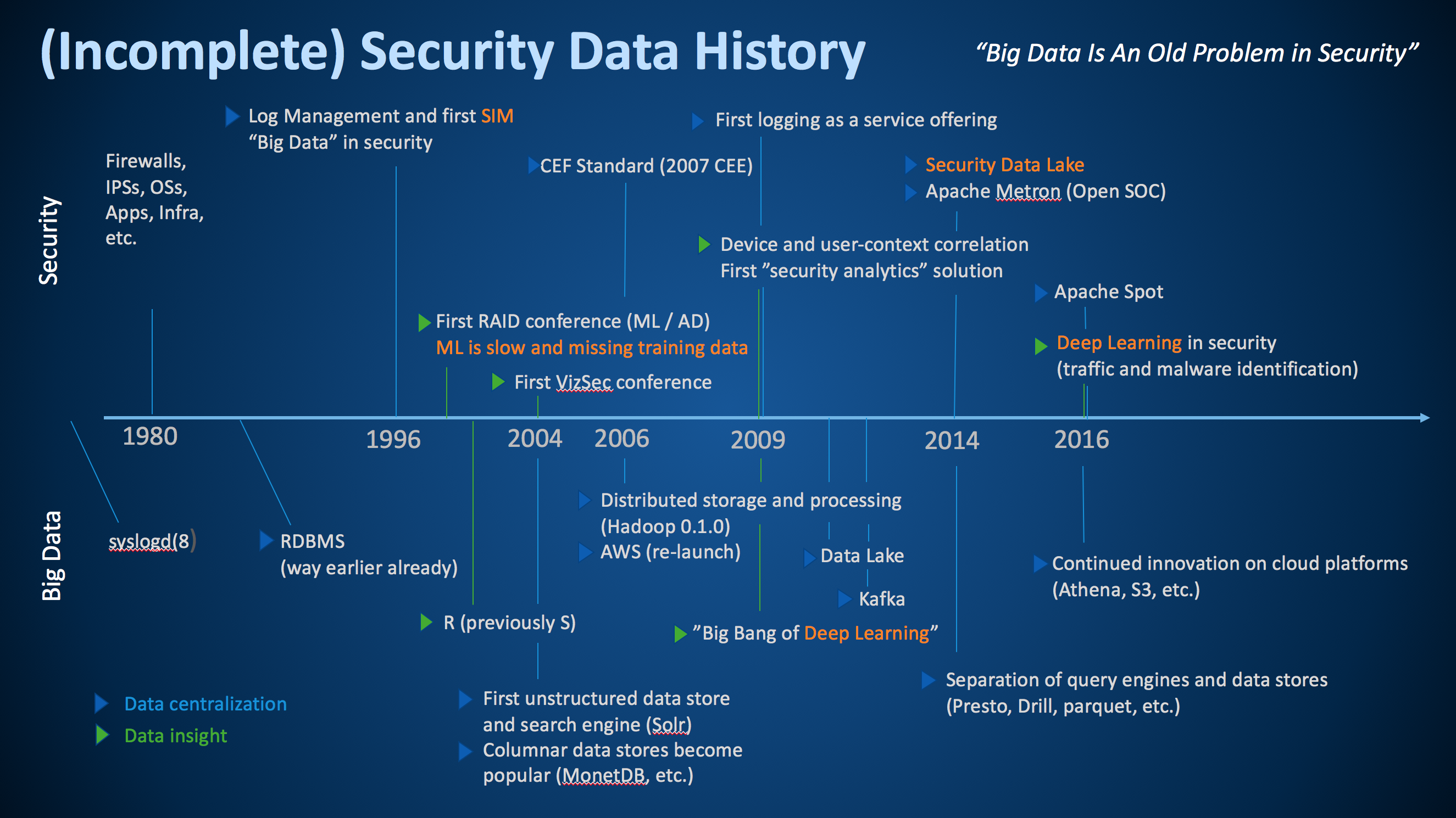
Earlier today I was giving the keynote at ACSAC 2017. This year’s theme of the conference is big data for security. As part of my keynote, I talked about the history of big data in security. Following is the slide I put together:

This is by no means a complete picture, but I tried to pull together some of the most important milestones along the security data journey. To help interpret the graph, the top part shows some of the most important developments in security, while the bottom shows the history in the big data world at large. I am including the big data world as without the developments in big data, security would not be where it is today.
In addition to distinguishing between security and big data developments, I am using blue and green triangles to differentiate between ‘data collection or centralization’ (blue) and ‘data insight’ (green) milestones. I had a hard time coming up with too many ‘data insight’ milestones in both big data and in security. Seems we have a bit more work to do in our industry.
Let me make a few remarks about the graph. I’d be curious about your thoughts also; please leave a comment.
- Security has been dealing with big data (variety, velocity, and volume) since 1996 – we just didn’t call it that back then.
- We have been trying to apply anomaly detection to (network) security data for a long time. Interestingly enough, we are still dealing with a lot of the same issues as we had back then; one of them is having access to good training data.
- We have been talking about security visualization for a long time. The first VizSec conference was held back in 2004. And in fact, we released the first versions of AfterGlow in early 2004.
- In 2006 we released the first common data format, the common event format (CEF). CEF was a vendor driven approach (I co-wrote the standard while at ArcSight). Later in 2007, I approached mitre to help us take the effort public under the CEE banner. Unfortunately, that effort wasn’t super successful. Later I rewrote CEF at Splunk and we called it the common information model (CIM). Now we also have Apache Spot that released yet another standard data format. Which standard are we going to use? Well, for my own purposes, none of these standards really made the cut and I wrote yet another field dictionary at Sophos (to be released). The other problem with these standards is that none of them cover semantics, only syntax!
- While deep learning had a big break through in 2009, we really only started using those algorithms in security in 2016. That’s probably a good thing. It’s just another machine learning algorithm that is actually really amazing at helping classify malware. But for a lot of other security problems it’s just not suited.
- In 2014 I wrote the first version of the security data lake booklet. Most of the challenges I address in there are still applicable today. One of the developments that has helped making data lakes more realistic, are developments like Apache Drill or PrestoDB; or in general, the separation of data storage (e.g., parquet) from the query engines. These developments allow us to query our data lake with many different storage formats (CSV, JSON, parquet, ORC, etc.). It still requires a master data record to understand what we have and let us manage schemas across data sources.
- Looking at database technologies, it is amazing to see what, for example, AWS has been providing with regards to tooling around data storage and access. Athena, RDS, S3, and to a lesser degree QuickSight, are fantastic tools to manage and explore large amounts of data. They provide the user with a lot of enterprise features out of the box, such as backups, fault tolerance, queueing, access control, etc.
What major milestones am I missing?
November 24, 2017
Last week I organized the 4th iteration of the Security Chat – an informal gathering of security people in Zurich where we talk about all type of security from cyber security to home security using systems online, and you can learn more here about this. The format are 10-15 minute presentations that anyone can submit for. In good tradition, we had a great line up again:
- Steve Micallef – OSINT and The New Perimeter – his tool is available for anyone to use at www.spiderfoot.net.
- Ero Carrera – The Many Types of Machine Learning.
Let’s not get carried away by the hype around deep learning. It’s great for some things, but not suited for many others. How about using Bayesian graph networks?
- Stefan Frei – Supply Chain Security in The Digital Age
Stefan gave us a bit to debate and think about when it comes to the security of the supply chain. Especially when it comes to Government procurement.
- Maxim Salomon – Foobar on Embedded Systems
Just how secure are our IoT devices out there? The presentation showed how insecure they really are. Even government grade security products!
- Jeroen Massar – Don’t Forget The Network
In his ‘no-slide’ presentation he made us remember that there are many aspects of networking that we tend to forget or a lot of people simply don’t know anymore. Things like BCP38, DNS RPC, etc.
- Sandra Tobler – Next Generation Multi Factor Authentication
More about the system that Sandra introduced can be found at: Futurae.com
October 22, 2017
After my latest blog post on “Machine Learning and AI – What’s the Scoop for Security Monitoring?“, there was a quick discussion on twitter and Shomiron made a good point that in my post I solely focused on supervised machine learning.
In simple terms, as mentioned in the previous blog post, supervised machine learning is about learning with a training data set. In contrast, unsupervised machine learning is about finding or describing hidden structures in data. If you have heard of clustering algorithms, they are one of the main groups of algorithms in unsupervised machine learning (the other being association rule learning).
There are some quite technical problems with applying clustering to cyber security data. I won’t go into details for now. The problems are related to defining distance functions and the fact that most, if not all, clustering algorithms have been built around numerical and not categorical data. Turns out, in cyber security, we mostly deal with categorical data (urls, usernames, IPs, ports, etc.). But outside of these mathematical problems, there are other problems you face with clustering algorithms. Have a look at this visualization of clusters that I created from some network traffic:
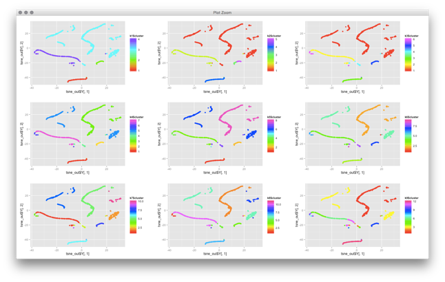
Some of the network traffic clusters incredibly well. But now what? What does this all show us? You can basically do two things with this:
- You can try to identify what each of these clusters represent. But the explainability of clusters is not built into clustering algorithms! You don’t know why something shows up on the top right, do you? You have to somehow figure out what this traffic is. You could run some automatic feature extraction or figure out what the common features are, but that’s generall not very easy. It’s not like email traffic will nicely cluster on the top right and Web traffic on the bottom right.
- You may use this snapshot as a baseline. In fact, in the graph you see individual machines. They cluster based on their similarity of network traffic seen (with given distance functions!). If you re-run the same algorithm at a later point in time, you could try to see which machines still cluster together and which ones do not. Sort of using multiple cluster snapshots as anomaly detectors. But note also that these visualizations are generally not ‘stable’. What was on top right might end up on the bottom left when you run the algorithm again. Not making your analysis any easier.
If you are trying to implement case number one above, you can make it a bit little less generic. You can try to inject some a priori knowledge about what you are looking for. For example, BotMiner / BotHunter uses an approach to separate botnet traffic from regular activity.
These are some of my thoughts on unsupervised machine learning in security. What are your use-cases for unsupervised machine learning in security?
PS: If you are doing work on clustering, have a look at t-SNE. It’s a clustering algorithm that does a multi-dimensional projection of your data into the 2-dimensional space. I have gotten incredible results with it. I’d love to hear from you if you have used the algorithm.