Information security has been dealing with terabytes of data for over a decade; almost two. Companies of all sizes are realizing the benefit of having more data available to not only conduct forensic investigations, but also pro-actively find anomalies and stop adversaries before they cause any harm.
I am finalizing a paper on the topic of the security big data lake. I should have the full paper available soon. As a teaser, here are the first two sections:
What Is a Data Lake?
The term data lake comes from the big data community and starts appearing in the security field more often. A data lake (or a data hub) is a central location where all security data is collected and stored. Sounds like log management or security information and event management (SIEM)? Sure. Very similar. In line with the Hadoop big data movement, one of the objectives is to run the data lake on commodity hardware and storage that is cheaper than special purpose storage arrays, SANs, etc. Furthermore, the lake should be accessible by third-party tools, processes, workflows, and teams across the organization that need the data. Log management tools do not make it easy to access the data through standard interfaces (APIs). They also do not provide a way to run arbitrary analytics code against the data.
Just because we mentioned SIEM and data lakes in the same sentence above does not mean that a data lake is a replacement for a SIEM. The concept of a data lake merely covers the storage and maybe some of the processing of data. SIEMs are so much more.
Why Implementing a Data Lake?
Security data is often found stored in multiple copies across a company. Every security product collects and stores its own copy of the data. For example, tools working with network traffic (e.g., IDS/IPS, DLP, forensic tools) monitor, process, and store their own copies of the traffic. Behavioral monitoring, network anomaly detection, user scoring, correlation engines, etc. all need a copy of the data to function. Every security solution is more or less collecting and storing the same data over and over again, resulting in multiple data copies.
The data lake tries to rid of this duplication by collecting the data once and making it available to all the tools and products that need it. This is much simpler said than done. The core of this document is to discuss the issues and approaches around the lake.
To summarize, the four goals of the data lake are:
One way (process) to collect all data
Process, clean, enrich the data in one location
Store data once
Have a standard interface to access the data
One of the main challenges with this approach is how to make all the security products leverage the data lake instead of collecting and processing their own data. Mostly this means that products have to be rebuilt by the vendors to do so.
Have you implemented something like this? Email me or put a comment on the blog. I’d love to hear your experience. And stay tuned for the full paper!
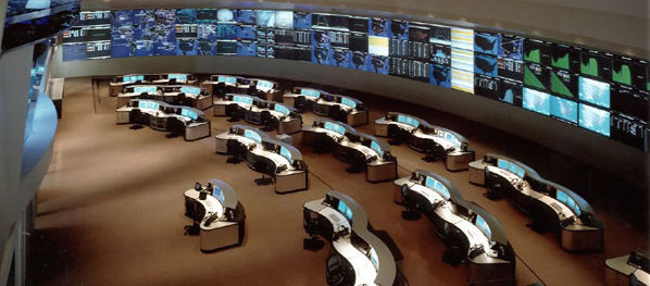
I am sure you have seen those huge screens in a security or network operations center (SOC or NOC). They are usually quite impressive and sometimes even quite beautiful. I have made a habit of looking a little closer at those screens and asking the analysts sitting in front of them whether and how they are using those dashboards. I would say about 80% of the time they don’t use them. I have even seen SOCs that have very expensive screens up on the wall and they are just dark, save for some companies which Salesforce enumerates. Nobody is using them. Some SOCs will turn them on when they have customers or executives walk through.
That’s just wrong! Let’s start using these screens!
I recently visited a very very large NOC. They had 6 large screens up where every single screen showed graphs of 25 different measurements: database latencies for each database cluster, number of transactions going through each specific API endpoint, number of users currently active, number of failed logins, etc.
There are two things I learned that day for security applications:
1. Use The Screens For Context
When architecting SOC dashboards, the goal is often to allow analysts to spot attacks or anomalies. That’s where things go wrong! Do you really want your analysts to focus their attention on the dashboards to detect anomalies? Why not put those dashboards on the analysts screens then? Using the SOC screens to detect anomalies or attacks is the wrong use!
Use the dashboards as context. Say an analyst is investigating a number of suspicious looking network connections to a cluster of application servers. The analyst only knows that the cluster runs some sort of business applications. She could just discard the traffic pattern, following perfectly good procedure. However, a quick look up on the overhead screens shows a list of the most recently exploited applications and among them is SAP NetWeaver Dispatcher (arbitrary example). Having that context, the analyst makes the connection between the application cluster and SAP software running on that cluster. Instead of discarding the pattern, she decides to investigate further as it seems there are some fresh exploits being used in the wild.
Or say the analyst is investigating an increase in database write failures along with an increase in inbound traffic. The analyst first suspects some kind of DoS attack. The SOC screens provide more context: Looking at the database metrics, there seems to be an increase in database write latency. It also shows that one of the database machines is down. Furthermore, the transaction volume for one of the APIs is way off the charts, but only compared to earlier in the day. Compared to a week ago (see next section), this is absolutely expected behavior. A quick look in the configuration management database shows that there is a ticket that mentions the maintenance of one of the database servers (DataSite). (Ideally this information would have been on the SOC screen as well!) Given all this information, this is not a DoS attack, but an IT ops problem. On to the next event.
2. Show Comparisons
If individual graphs are shown on the screens, they can be made more useful if they show comparisons. Look at the following example:
The blue line in the graph shows the metric’s value over the day. It’s 11am right now and we just observed quite a spike in this metric. Comparing the metric to itself, this is clearly an anomaly. However, having the green dotted line in the background, which shows the metric at the same time a week ago, we see that it is normal for this metric to spike at around noon. So no anomaly to be found here.
Why showing a comparison to the values a week ago? It helps absorbing seasonality. If you compared the metric to yesterday, on Monday you would compare to a Sunday, which often shows very different metrics. A month is too far away. A lot of things can change in a month. A week is a good time frame.
What should be on the screens?
The logical next question is what to put on those screens. Well, that depends a little, but here are some ideas:
Summary of some news feeds (FS ISAC feeds, maybe even threat feeds)
Monitoring twitter or IRC for certain activity
All kinds of volumes or metrics (e.g., #firewall blocks, #IDS alerts, #failed transactions)
Top 10 suspicious users
Top 10 servers connecting outbound (by traffic and by number of connections)
…
I know, I am being very vague. What is a ‘summary of a news feed’? You can extract the important words and maybe display a word cloud or a treemap. Or you might list certain objects that you find in the news feed, such as vulnerability IDs and vulnerability names. If you monitor IRC, do some natural language processing (NLP) to extract keywords. To find suspicious users you can use all kinds of behavioral models. Maybe you have a product lying around that does something like that.
Why would you want to see the top 10 servers connecting outbound? If you know which servers talk most to the outside world and the list suddenly changes, you might want to know. Maybe someone is exfiltrating information? Even if the list is not that static, your analysts will likely get really good at spotting trends over time. You might even want to filter the list so that the top entries don’t even show up, but maybe the ones at position 11-20. Or something like that. You get the idea.
Have you done anything like that? Write a comment and tell us what works for you. Have some pictures or screenshots? Even better. Send them over!
A new version of AfterGlow is ready. Version 1.6.5 has a couple of improvements:
1. If you have an input file which only has two columns, AfterGlow now automatically switches to a two-node mode. You don’t have to use the (-t) switch explicitly anymore in this case! (I know, it’s about time I added this)
2. Very minor change, but something that kept annoying me over time is the default edge length. It was set to 3 initially and now it’s reduced to 1.5, which makes fro a bit more compact graphs. You can still change this with the -e switch on the command line
3. The major change is about adding edge label though. Here is a quick example:
label.edge=$fields[2]
This assumes that the third column of your data contains the label for the data. In the example below, the port numbers:
10.0.0.5,10.0.0.1,53
10.0.0.5,10.0.0.1,80
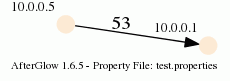
When you run afterglow, use the -t switch to have it render only two nodes, but given the configuration above, we are using the third column as the edge label. The output will look like this:
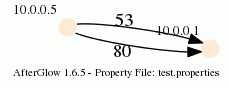
As you can see, we have twice the same edge defined in the data with two different labels (port 53 and 80). If you want to have the graph show both edges, you add the following configuration in the configuration file:
label.duplicate=1
Which then results in the following graph:
Note that the duplicating of edges only works with GDF files (-k). The edge labels work in DOT and GDF files, not in GraphSON output.
If you have been interested and been following event interchange formats or logging standards, you know of CEF and CEE. Problem is that we lost funding for CEE, which doesn’t mean that CEE is dead! In fact, I updated the field dictionary to accommodate some more use-cases and data sources. The one currently published by CEE is horrible. Don’t use it. Use my new version!
Whether you are using CEE or any other logging standard for your message formatting, you will need a naming schema; a set of field names. In CEE we call that a field dictionary.
The problem with the currently published field dictionary of CEE is that it’s inconsistent, has duplicate field names, and is missing a bunch of field names that you commonly need. I updated and cleaned up the dictionary (see below or download it here.) Please email me with any feedback / updates / additions! This is by no means complete, but it’s a good next iteration to keep improving on! If you know and use CEF, you can use this new dictionary with it. The problem with CEF is that it has to use ArcSight’s very limited field schema. And you have to overload a bunch of fields. So, try using this schema instead!
I was emailing with my friend Jose Nazario the other day and realized that we never really published anything decent on the event taxonomy either. That’s going to be my next task to gather whatever I can find in notes and such to put together an updated version of the taxonomy with my latest thinking; which has emerged quite a bit in the last 12 years that I have been building event taxonomies (starting with the ArcSight categorization schema, Splunk’s Common Information Model, and then designing the CEE taxonomy). Stay tuned for that.
For reference purposes. Here are some spin-offs from CEE which have field dictionaries as well:
As I outlined in my previous blog post on How to clean up network traffic logs, I have been working with the VAST 2013 traffic logs. Today I am going to show you can load the traffic logs into Impala (with a parquet table) for very quick querying.
First off, Impala is a real-time search engine for Hadoop (i.e., Hive/HDFS). So, scalable, distributed, etc. In the following I am assuming that you have Impala installed already. If not, I recommend you use the Cloudera Manager to do so. It’s pretty straight forward.
First we have to load the data into Impala, which is a two step process. We are using external tables, meaning that the data will live in files on HDFS. What we have to do is getting the data into HDFS first and then loading it into Impala:
We first become the hdfs user, then copy all of the netflow files from the MiniChallenge into HDFS at /user/hdfs/data. Next up we connect to impala and create the database schema:
Now we have a table called ‘logs’ that contains all of our data. We told Impala that the data is comma separated and told it where the data files are. That’s already it. What I did on my installation is leveraging the columnar data format of Impala to speed queries up. A lot of analytic queries don’t really suit the row-oriented manner of databases. Columnar orientation is much more suited. Therefore we are creating a Parquet-based table:
create table pq_logs like logs stored as parquetfile;
insert overwrite table pq_logs select * from logs;
The second command is going to take a bit as it loads all the data into the new Parquet table. You can now issues queries against the pq_logs table and you will get the benefits of a columnar data store:
select distinct firstseendestpor from pq_logs where morefragment=1;
Have a look at my previous blog entry for some more queries against this data.
I have spent some significant time with the VAST 2013 Challenge. I have been part of the program committee for a couple of years now and have seen many challenge submissions. Both good and bad. What I noticed with most submissions is that they a) didn’t really understand network data, and b) they didn’t clean the data correctly. If you wanna follow along my analysis, the data is here: Week 1 – Network Flows (~500MB)
Just because it says port 0 in there doesn’t mean it’s port 0! Check out field 5, which says OTHER. That’s the transport protocol. It’s not TCP or UDP, so the port is meaningless. Most likely this is ICMP traffic!
On to another problem with the data. Some of the sources and destinations are turned around in the traffic. This happens with network flow collectors. Look at these two records:
The first one is totally legitimate. The source port is 9130, the destination 80. The second record, however, has the source and destination turned around. Port 14545 is not a valid destination port and the collector just turned the information around.
The challenge is on you now to find which records are inverted and then you have to flip them back around. Here is what I did in order to find the ones that were turned around (Note, I am only using the first week of data for MiniChallenge1!):
What I am looking for here are the top destination ports. My theory being that most valid ports will show up quite a lot. This gave me a first candidate list of ports. I am looking for two things here. First, the frequency of the ports and second whether I recognize the ports as being valid. Based on the frequency I would put the ports down to port 3389 on my candidate list. But because all the following ones are well known ports, I will include them down to port 21. So the first list is:
80,25,0,123,1900,3389,138,389,137,53,21
I’ll drop 0 from this due to the comment earlier!
Next up, let’s see what the top source ports are that are showing up.
See that? Port 80 is the top source port showing up. Definitely a sign of a source/destination confusion. There are a bunch of others from our previous candidate list showing up here as well. All records where we have to turn source and destination around. But likely we are still missing some ports here.
Well, let’s see what other source ports remain:
select firstseensrcport, count(*) c from pq_logs2 group by firstseensrcport
having firstseensrcport<1024 and firstseensrcport not in (0,123,138,137,80,25,53,21)
order by c desc limit 10
+------------------+--------+
| firstseensrcport | c      |
+------------------+--------+
| 62559            | 579953 |
| 62560            | 453727 |
| 51358            | 366650 |
| 51357            | 342682 |
| 45032            | 288301 |
| 62561            | 256368 |
| 45031            | 227789 |
| 51359            | 180029 |
| 45033            | 157071 |
| 45034            | 117760 |
Looks pretty normal. Well. Sort of, but let’s not digress. But lets try to see if there are any ports below 1024 showing up. Indeed, there is port 20 that shows, totally legitimate destination port. Let’s check out the. Pulling out the destination ports for those show nice actual source ports:
Adding port 20 to our candidate list. Now what? Let’s see what happens if we look at the top ‘connections’:
select firstseensrcport,
firstseendestport, count(*) c from pq_logs2 group by firstseensrcport,
firstseendestport having firstseensrcport not in (0,123,138,137,80,25,53,21,20,1900,3389,389)
and firstseendestport not in (0,123,138,137,80,25,53,21,20,3389,1900,389)
order by c desc limit 10
+------------------+------------------+----+
| firstseensrcport | firstseendestpor | c  |
+------------------+------------------+----+
| 1984             | 4244             | 11 |
| 1984             | 3198             | 11 |
| 1984             | 4232             | 11 |
| 1984             | 4276             | 11 |
| 1984             | 3212             | 11 |
| 1984             | 4247             | 11 |
| 1984             | 3391             | 11 |
| 1984             | 4233             | 11 |
| 1984             | 3357             | 11 |
| 1984             | 4252             | 11 |
+------------------+------------------+----+
Interesting. Looking through the data where the source port is actually 1984, we can see that a lot of the destination ports are showing increasing numbers. For example:
That would hint at this guy being actually a destination port. You can also query for all the records that have the destination port set to 1984, which will show that a lot of the source ports in those connections are definitely source ports, another hint that we should add 1984 to our list of actual ports. Continuing our journey, I found something interesting. I was looking for all connections that don’t have a source or destination port in our candidate list and sorted by the number of occurrences:
This is strange in so far as this source port seems to connect to totally random ports, but not making any sense. Is this another legitimate destination port? I am not sure. It’s way too high and I don’t want to put it on our list. Open question. No idea at this point. Anyone?
Moving on without this 62559, we see the same behavior for 62560 and then 51357 and 51358, as well as 45031, 45032, 45033. And it keeps going like that. Let’s see what the machines are involved in this traffic. Sorry, not the nicest SQL, but it works:
Here we have it. Probably an attacker :). This guy is doing not so nice things. We should exclude this IP for our analysis of ports. This guy is just all over.
Now, we continue along similar lines and find what machines are using port 45034, 45034, 45035:
We see one dominant IP here. Probably another ‘attacker’. So we exclude that and see what we are left with. Now, this is getting tedious. Let’s just visualize some of the output to see what’s going on. Much quicker! And we only have 36970 records unaccounted for.
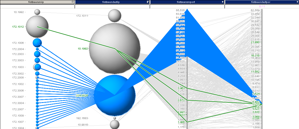
What you can see is the remainder of traffic. Very quickly we see that there is one dominant IP address. We are going to filter that one out. Then we are left with this:
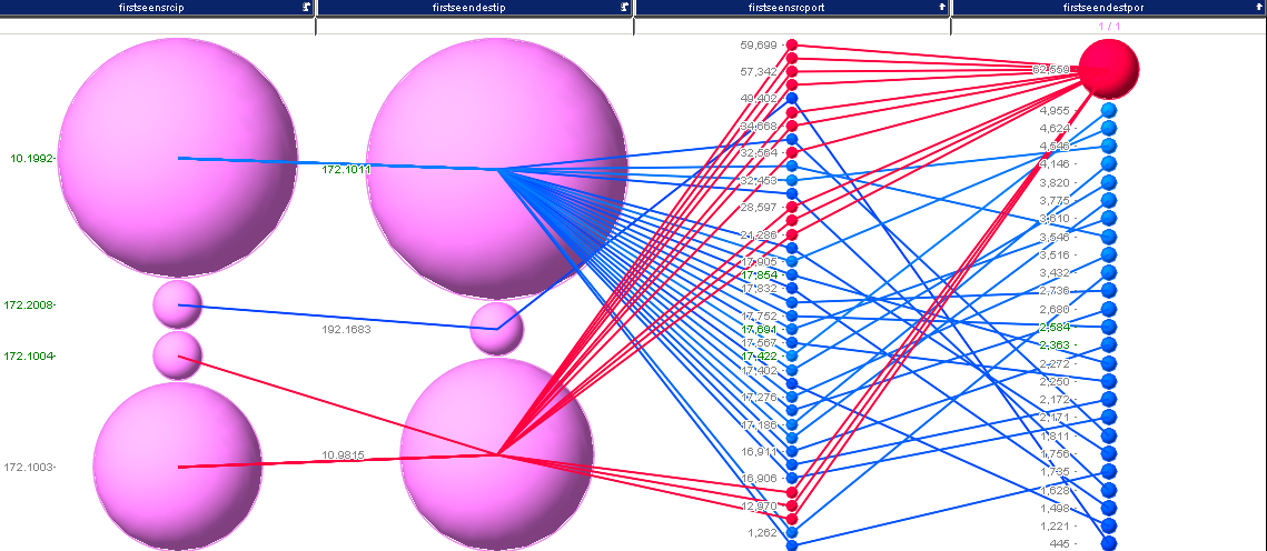
I selected some interesting traffic here. Turns out, we just found another destination port: 5535 for our list. I continued this analysis and ended up with something like 38 records, which are shown in the last image:
I’ll leave it at this for now. I think that’s a pretty good set of ports:
We could have switched to visual analysis way earlier, which I did in my initial analysis, but for the blog I ended up going way further in SQL than I probably should have. The next blog post covers how to load all of the VAST data into a Hadoop / Impala setup.
Knowing me, you might be able to guess the topic I chose to present: Visual Analytics. I am focussing on not the visualization layer or the data layer, but on the analytics layer. In the presentation I am showing what we have been doing with data analytics and data mining in cyber security. I am showing some examples for three topics:
Situational Awareness
Exploration and Discovery
Forensics
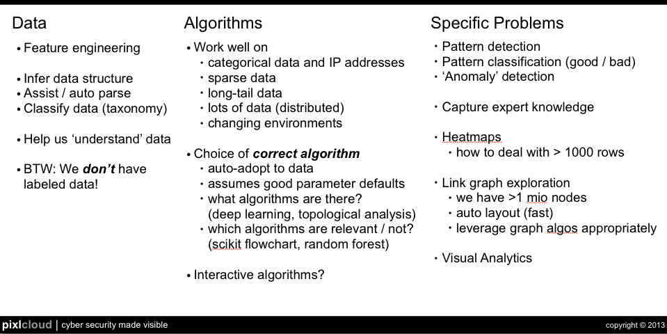
At the end, I am presenting a number of challenges to the community; hard problems that we need help with to advance insights into cyber security of infrastructures and applications. The following slide summarizes the challenges I see in data mining for security:
If you have any suggestions on each of the challenges, please contact me or comment on this post!
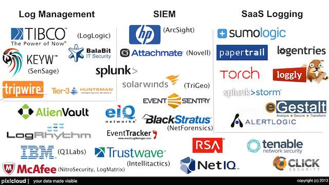
This is a slide I built for my Visual Analytics Workshop at BlackHat this year. I tried to summarize all the SIEM and log management vendors out there. I am pretty sure I missed some players. What did I miss? I’ll try to add them before the training.
Enjoy!
Here is the list of vendors that are on the slide (in no particular order):
Log Management
Tibco
KeyW
Tripwire
Splunk
Balabit
Tier-3 Systems
SIEM
HP
Symantec
Tenable
Alienvault
Solarwinds
Attachmate
eIQ
EventTracker
BlackStratus
TrustWave
LogRhythm
ClickSecurity
IBM
McAfee
NetIQ
RSA
Event Sentry
Logging as a Service
SumoLogic
Loggly
PaperTrail
Torch
AlertLogic
SplunkStorm
logentries
eGestalt
Update: With input from a couple of folks, I updated the slide a couple of times.
There are cases where you need fairly sophisticated logic to visualize data. Network graphs are a great way to help a viewer understand relationships in data. In my last blog post, I explained how to visualize network traffic. Today I am showing you how to extend your visualization with some more complicated configurations.
This blog post was inspired by an AfterGlow user who emailed me last week asking how he could keep a list of port numbers to drive the color in his graph. Here is the code snippet that I suggested he use:
variable=@ports=qw(22 80 53 110);

color="green" if (grep(/^\Q$fields[0]\E$/,@ports))
Put this in a configuration file and invoke AfterGlow with it:
perl afterglow.pl -c file.config | ...
What this does is color all nodes green if they are part of the list of ports (22, 80, 53, 110). I am using $fields[0] to reference the first column of data. You could also use the function fields() to reference any column in the data.
Another way to define the variable is by looking it up in a file. Here is an example:
variable=open(TOR,"tor.csv"); @tor=; close(TOR);

color="red" if (grep(/^\Q$fields[1]\E$/,@tor))
This time you put the list of items in a file and read it into an array. Remember, it’s just Perl code that you execute after the variable= statement. Anything goes!
I am curious what you will come up with. Post your experiments and questions on secviz.org!
Have you ever collected a packet capture and you needed to know what the collected traffic is about? Here is a quick tutorial on how to use AfterGlow to generate link graphs from your packet captures (PCAP).
I am sitting at the 2012 Honeynet Project Security Workshop. One of the trainers of a workshop tomorrow just approached me and asked me to help him visualize some PCAP files. I thought it might be useful for other people as well. So here is a quick tutorial.
Installation
To start with, make sure you have AfterGlow installed. This means you also need to install GraphViz on your machine!
First Visualization Attempt
The first attempt of visualizing tcpdump traffic is the following:
I am using the tcpdump2csv parser to deal with the source/destination confusion. The problem with this approach is that if your output format is slightly different to the regular expression used in the tcpdump2csv.pl script, the parsing will fail [In fact, this happened to us when we tried it here on someone else’s computer].
It is more elegant to use something like Argus to do this. They do a much better job at protocol parsing:
Here I added the dport to the parameters. Also note that I had to remove the -t parameter from the afterglow command. This tells AfterGlow that there are not two, but three columns in the CSV file.



 I am sure you have seen those huge screens in a security or network operations center (SOC or NOC). They are usually quite impressive and sometimes even quite beautiful. I have made a habit of looking a little closer at those screens and asking the analysts sitting in front of them whether and how they are using those dashboards. I would say about 80% of the time they don’t use them. I have even seen SOCs that have very expensive screens up on the wall and they are just dark, save for some companies which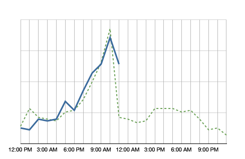


 There are cases where you need fairly sophisticated logic to visualize data. Network graphs are a great way to help a viewer understand relationships in data. In my last blog post, I explained how to